Dissecting the Bloch Sphere

December 26, 2022

Learning quantum computing typically involves learning about the Bloch sphere, a representation of a qubit state as a point on the unit sphere. However, most sources don’t dig into how it really works, mathematically speaking. For example, neither the Qiskit textbook nor Mike & Ike attempt to explain the formula for the Bloch sphere to readers, only dumping the formula and saying “have fun!”

This post focuses on how the beloved Bloch sphere emerges. I am summarizing my understanding of a 1990 paper by Urbantke and a 2001 paper by Mosseri and Dandoloff.

Emergence of the 3-Sphere

An arbitrary single-qubit state is typically defined as

\[ \begin{align} | \psi \rangle &= \begin{bmatrix}z_1 \\ z_2\end{bmatrix}, \text{ where } z_1, z_2 \in \mathbb{C} \text{ and } |z_1|^2 + |z_2|^2 = 1 \end{align} \]

That doesn’t provide much geometric intuition. To help, let’s define

\[ \begin{align} z_1 &= x_1 + x_2 i \\ z_2 &= x_3 + x_4 i,\text{ where } x_i \in \mathbb{R} \\ \end{align} \]

Now the set of all $| \psi \rangle$ above is isomorphic to the set of the following:

\[ \begin{align} \vec{v} &= \begin{bmatrix}x_1 \\ x_2 \\ x_3 \\ x_4\end{bmatrix},\text{ where } x_1^2 + x_2^2 + x_3^2 + x_4^2 = 1 \end{align} \]

Much better! The set of all $\vec{v}$s is just the 3-sphere, aka $S^3$, aka a unit hypersphere in 4D space! But there’s a catch…

Global Phase

According to the postulates of quantum mechanics, a state $| \psi \rangle$ has the exact same distribution of measurements as $e^{i\theta}|\psi\rangle$ (where $\theta \in \mathbb{R}$) for any measurement operator¹. Even in a composite state, you can factor out that $e^{i\theta}$ from the state of an individual qubit, and that factor doesn’t affect measurements of the whole system either. For that reason, I’ve seen physicists call that global phase factor $e^{i\theta}$ “unimportant” — poor guy!

What does global phase look like on our friend the 3-sphere? We can write $e^{i\theta}|\psi\rangle$ as

\[ e^{i\theta}|\psi\rangle = (\cos \theta)|\psi\rangle + (\sin \theta)i|\psi\rangle \]

Now, we could write that as the following in our isomorphic world of $\mathbb{R}^4$ if we had an operator $J$ that behaved the same as multiplication by $i$ in $\mathbb{C}^2$:

\[ \vec{v}_\theta = (\cos \theta)\vec{v} + (\sin \theta)J\vec{v} \]

What is $J$? We can define

\[ J\begin{bmatrix}x_1 \\ x_2 \\ x_3 \\ x_4\end{bmatrix} = \begin{bmatrix}-x_2 \\ x_1 \\ -x_4 \\ x_3\end{bmatrix} \]

It turns out that $\vec{v}_\theta$ defines a circle in 4D space! That may make some intuitive sense given that $e^{i\theta}$ is a circle in the complex plane, but geometrically, why is that true? It turns out that $\vec{v}$ and $J\vec{v}$ are orthogonal because $\vec{v}\cdot J\vec{v} = 0$, thus $a\vec{v} + bJ\vec{v}$ with $a,b \in \mathbb{R}$ defines a 2D plane centered on the origin. $\vec{v}_\theta$ is just a circle on that plane!

A figure here would be nice, but it’s hard to see 4D. So to show this, I have drawn the circle in 4D and then done a stereographic projection down to 3D space. Here’s the result (the aforementioned plane is approximately your screen, and the axes shown are for 3D space):

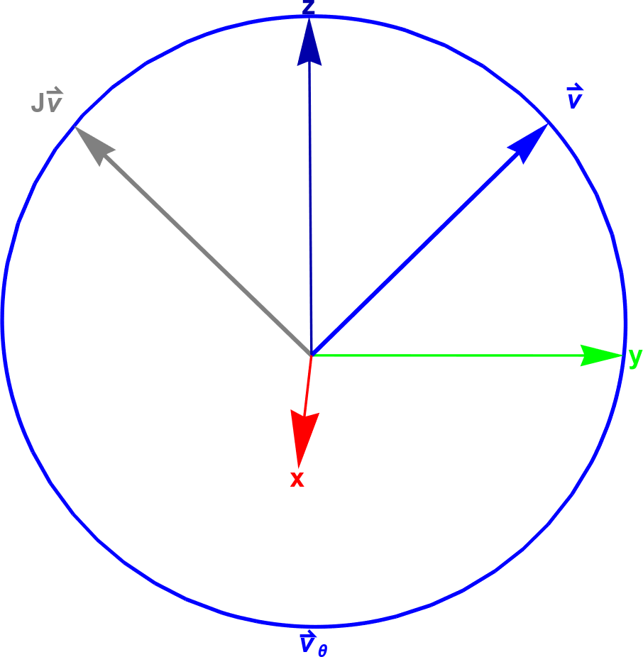
Fun observation: this circle must be a great circle of $S^3$, since it is the intersection of the aforementioned plane and $S^3$. Why? Both $\vec{v}_\theta$ and $S^3$ have the same radius (1) and the same center point (the origin).

Stereographic Trolling

The figure above produced by a stereographic projection from 4D into 3D looks nice because I cherrypicked $\vec{v}$ to make it look nice. What if I also plot a typical other point $\vec{w}$ from the surface of $S^3$?

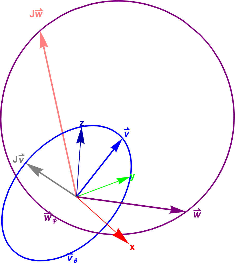
What the heck is that? $\vec{w}$ and $J\vec{w}$ aren’t even orthogonal in this projection, and how are both $\vec{v}_\theta$ and $\vec{w}_\phi$ unit circles when $\vec{w}_\phi$ is so much bigger? The projection is really bulldozing any geometric intuition here².

This 4D view makes for a poor visualization for qubit states because that third degree of freedom for $S^3$ puts us in 4D space, and we need to project to 3D to actually look at the 4D geometry. What if we discarded that third degree of freedom and collapsed each of these great circles to a point on the unit sphere instead? Roughly speaking, that’s the Hopf fibration.

The Hopf Fibration

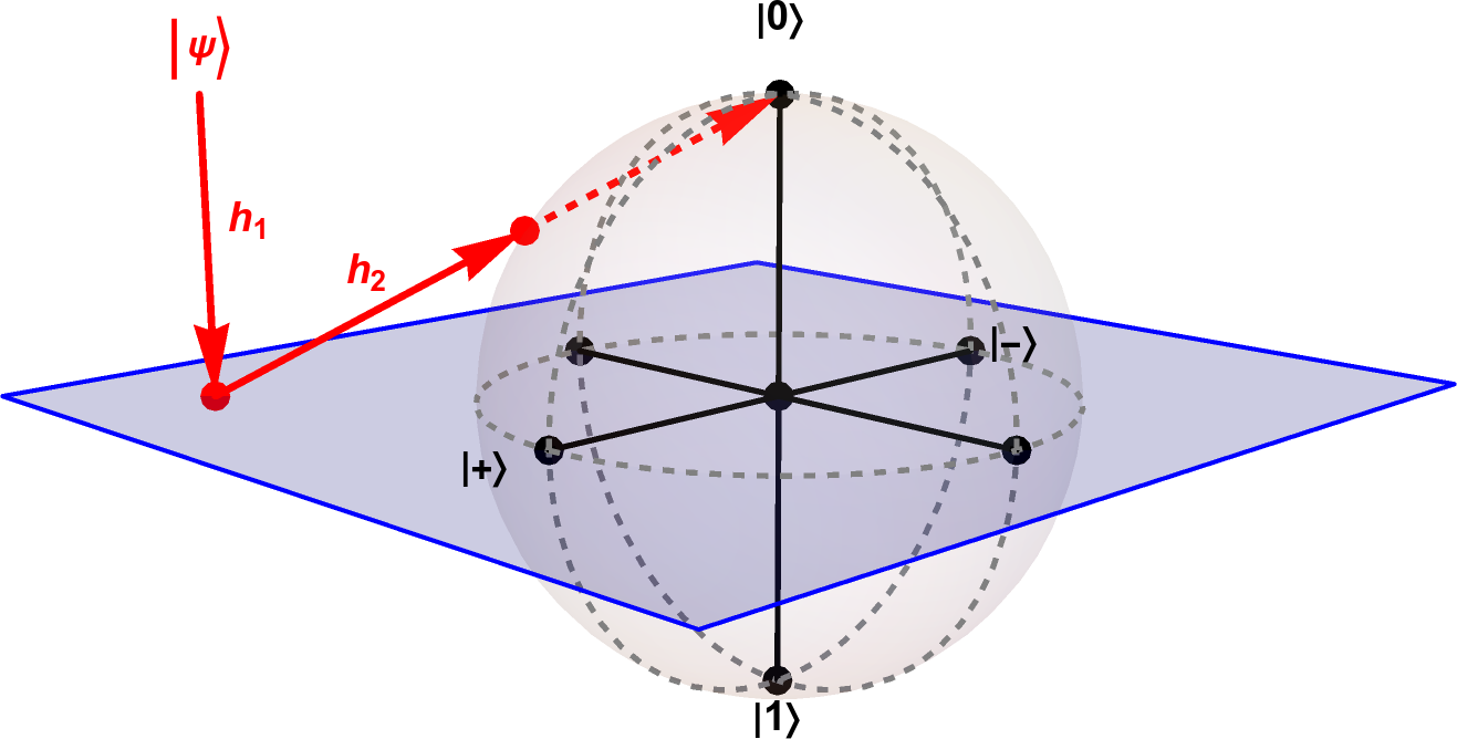
Intuitively, we want to to represent the two degrees of freedom we actually care about in a qubit state as a sphere (which has two degrees of freedom) but without the unhelpful third degree of freedom that lands us in 4D (global phase). The Hopf fibration can help with this. Mosseri and Dandoloff represent the Hopf fibration as the composition of two maps:

1. $h_1$, which maps a qubit state $|\psi\rangle$ into 2D space
2. $h_2$, which maps a point in 2D space to a point on the unit sphere in 3D using an inverse stereographic projection

Here’s a diagram:

Let’s dive into these maps one by one.

Mapping Qubit State into 2D ($h_1$)

The definition of this first map is simply (using the $z_1,z_2$ amplitudes defined above):

\[ h_1 = (z_1/z_2)^* \]

To get an idea of what this does, let’s re-parameterize $|\psi\rangle$ with $\theta,\phi,\gamma \in \mathbb{R}$ as follows:

\[ \begin{align} z_1 &= e^{i\gamma}\cos(\theta/2) \\ z_2 &= e^{i(\gamma + \phi)}\sin(\theta/2) \end{align} \]

This parameterization works because it can express all values of $z_1, z_2$ yet no choices of parameters can violate $|z_1|^2 + |z_2|^2 = 1$. This parameterization is pretty arbitrary but chosen so that we match the final resulting Bloch vector in Mike & Ike. (For example, the division by 2 in the trig functions will come in handy later.)

Now if we apply $h_1$ to $|\psi\rangle$: \[ \begin{align} h_1(z_1, z_2) &= \left(\frac{e^{i\gamma}\cos(\theta/2)}{e^{i(\gamma + \phi)}\sin(\theta/2)}\right)^* \\ &= \left(\frac{\cos(\theta/2)}{e^{i\phi}\sin(\theta/2)}\right)^* \\ &= e^{i\phi}\cot(\theta/2) \end{align} \] We can make a couple of handy observations from this: first, that division in $h_1$ is useful because it ‘cancels out’ global phase. Second, it produces a wonderful polar form! In the following figure, I plot the complex plane for some values of $\theta$ with $\phi$ free:

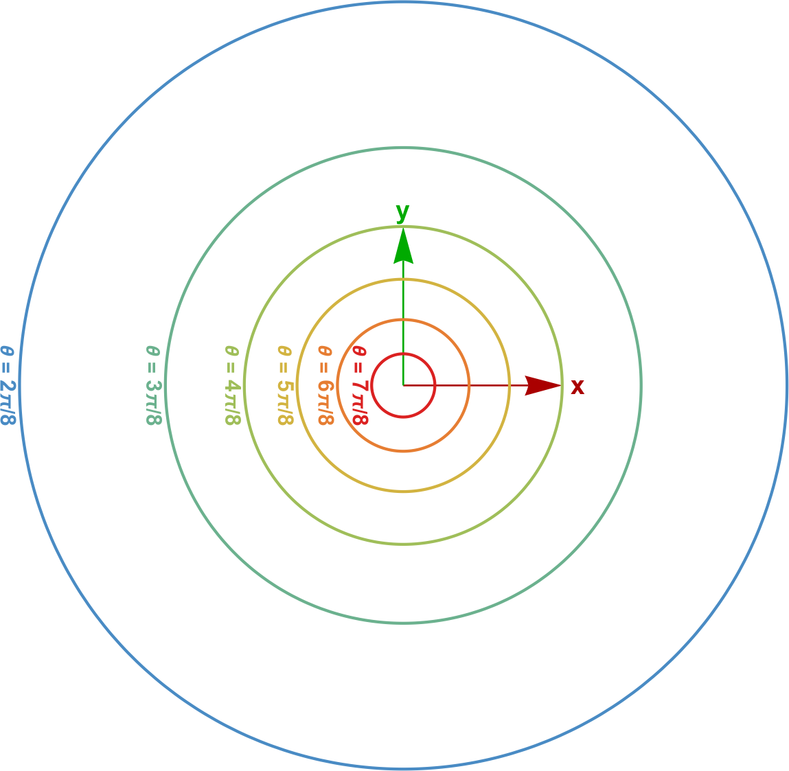
Looking at this example closely, you might notice it looks like a stereographic projection of some circles of latitude of the unit sphere onto a (2D) plane. Okay, that’s very specific, so you might not notice that, but it’s true:

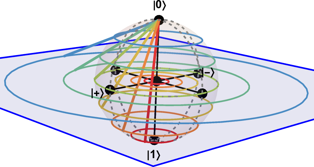
This leads to the second map, $h_2$…

Mapping 2D Points into 3D ($h_2$)

The second map $h_2$ is defined as an inverse stereographic projection from 2D back onto the surface of a sphere in 3D.

To get this to work, we re-interpret the complex result of $h_1$ as some coordinates in $\mathbb{R}^2$. Specifically, in our parameterization from above, \[ e^{i\phi}\cot(\theta/2) \Rightarrow (X,Y) = (\cos\phi\cot(\theta/2), \sin\phi\cot(\theta/2)) \] If we use the north pole of the sphere as the projection pole, and plug the above coordinates into the inverse stereographic projection equations from Wikipedia \[ (x,y,z) = \frac{1}{X^2 + Y^2 + 1}(2X, 2Y, X^2+Y^2-1) \] We get the following after applying some trig identities (including the double-angle identities, which eliminate the division of $\theta$ by two): \[ (x,y,z) = (\sin\theta\cos\phi, \sin\theta\sin\phi, \cos\theta) \] What do you know, that’s exactly the Bloch vector given by Mike & Ike in Section 4.2! It’s also the equation for a sphere in spherical coordinates! Believe it or not, it’s also the same as the expectation values of Pauli X, Y, and Z respectively, as Mosseri and Dandoloff point out: \[ (x,y,z) = (\langle\psi|\sigma_x|\psi\rangle, \langle\psi|\sigma_y|\psi\rangle, \langle\psi|\sigma_z|\psi\rangle) \]

Conclusion

In this post, I’ve tried my hand at explaining the Hopf fibration within the context of a single-qubit state. But the Hopf fibration is a beautiful construction in itself regardless of quantum anything, so don’t let me mislead you; there are some nice visualizations out there showing how great circles on $S^3$ are mapped to points on $S^2$, if you’re interested.

But even in quantum-world, the Hopf fibration applies to more than just one qubit: Mosseri and Dandoloff actually apply the Hopf fibration of $S^7$ to two-qubit states. They use a similar construction as theirs for $S^3$ that I’ve repeated above, except that $h_1$ takes the quotient of quaternions instead of complex numbers.

Finally, although this post talks about how to map states to points on the Bloch sphere, why do unitary matrices (quantum gates) map so well onto rotations on the Bloch sphere? The answer to that question is related to the fact that $SU(2)$ is a double cover of $SO(3)$ — that is, there are two different $2\times 2$ unitary matrices with determinant 1 for every proper 3D rotation. But that is the subject of another blog post in itself³.